Showing posts with label Performance tuning. Show all posts

Monday, July 21, 2014

PASS Data Arch VC presents SQL Server MVP Grant Fritchey - How to Build a Database Deployment Pipeline

Please come join the Data Architecture VC this Wednesday to get info from MVP Grant about Database Deployment something all DBAs should be doing to work with developers.

Grant Fritchey – Microsoft MVP

July 23, 2014 Noon CST

How to Build a Database Deployment Pipeline.

The pace of business accelerates fairly continuously and application development moves right with it. But we’re still trying to deploy databases the same way we did 10 years ago. This session addresses the need for changes in organizational structure, process and technology necessary to arrive at a nimble, fast, automatable and continuous database deployment process. We’ll use actual customer case studies to illustrate both the common methods and the unique context that led to a continuous delivery process that is best described as a pipeline. You will learn how to customize common practices and tool sets to build a database deployment pipeline unique to your environment in order to speed your own database delivery while still protecting your organization’s most valuable asset, its data.

Speaker Bio:

Grant Fritchey, SQL Server MVP, works for Red Gate Software as Product Evangelist. In his time as a DBA and developer, he has worked at three failed dot–coms, a major consulting company, a global bank and an international insurance & engineering company. Grant volunteers for the Professional Association of SQL Server Users (PASS). He is the author of the books SQL Server Execution Plans (Simple-Talk

Webinar Link Click here   https://attendee.gotowebinar.com/register/3676956357735772161

Tuesday, July 8, 2014

Upcoming Free PASS VC Webcasts

Here is a list of upcoming webcast presented by various PASS Virtual Chapters that are always free. Some are recorded to view later.


Database Administration VC

Date: July 9

Noon Mountainhttp://www.timeanddate.com/worldclock/fixedtime.html?msg=PASS+DBA+Virtual+Chapter&iso=20140709T12&p1=75

Topic: How to be a great DBA– sponsored by Dell Software

Registration: You must register if you want to attend. You can register at

https://attendee.gotowebinar.com/register/5111261580659448577

When you register, you will receive a link to the meeting. All registrants will be included in a drawing for a $50 Amazon gift card.

Presenter: Jeff Garbus

Abstract: This presentation describes the tasks a DBA needs to perform to do a great job. Formal training classes and certifications only take you so far; this session talks from experience about everything from preventive maintenance to planning to scaling to communication. Great for beginner to intermediate DBAs, as well as Developers who think this is a direction in which they might want to move.

Bio: Jeff Garbus is a well-known author, lecturer and consultant with more than 20 years of expertise in architecture, tuning and the administration of Microsoft SQL Server, Sybase ASE, Oracle, and other databases. Jeff has assisted clients of all sizes, from .com startups to the most demanding F100 clients. His specialty has always been maximizing database performance for his clients. Jeff has recently released his 16th book: Microsoft Transact SQL – The Definitive Guide. Jeff is also the founder and CEO of Soaring Eagle Consulting, a consulting and management consulting firm specializing in all aspects of database and information management. http://mssqlperformance.blogspot.com/


DBA Fundamental VC


WHAT       Rolling Upgrades, The Easy Way!

WHEN:      Tuesday, August 5,   11:00 AM – 12:00 PM CDT

WHO:        Argenis Fernandez

WHERE:   https://attendee.gotowebinar.com/register/998862692698291202

In this session we will discuss how to perform upgrades while maintaining high availability of your SQL server infrastructure by leveraging rolling upgrades. We will review how to use database mirroring or AlwaysOn Availability Groups for this, along with a simpler version using Log Shipping. This is a demo-intensive session that you won't want to miss. 

There will be a drawing for a $25  Amazon gift card at the end of the meeting.  A winner will be randomly chosen from all those in attendance for the whole webcast who provide their email address.


Data Architecture VC


Grant Fritchey – Microsoft MVP

July 23, 2014 Noon CST

How to Build a Database Deployment Pipeline.

The pace of business accelerates fairly continuously and application development moves right with it. But we’re still trying to deploy databases the same way we did 10 years ago. This session addresses the need for changes in organizational structure, process and technology necessary to arrive at a nimble, fast, automatable and continuous database deployment process. We’ll use actual customer case studies to illustrate both the common methods and the unique context that led to a continuous delivery process that is best described as a pipeline. You will learn how to customize common practices and tool sets to build a database deployment pipeline unique to your environment in order to speed your own database delivery while still protecting your organization’s most valuable asset, its data.

Speaker Bio:

Grant Fritchey, SQL Server MVP, works for Red Gate Software as Product Evangelist. In his time as a DBA and developer, he has worked at three failed dot–coms, a major consulting company, a global bank and an international insurance & engineering company. Grant volunteers for the Professional Association of SQL Server Users (PASS). He is the author of the books SQL Server Execution Plans (Simple-Talk

Webinar https://attendee.gotowebinar.com/register/3676956357735772161


Virtualization VC


Wed, Jul 09 2014 10:00 Mountain Daylight Time


SQL Server Virtualization 301

RSVP: https://attendee.gotowebinar.com/register/6360531090119570945

SQL SERVER VIRTUALIZATION 301

Can you objectively demonstrate that your SQL Servers are running the same or better after they were virtualized than when they were physical servers? Do you have your key system monitoring in place so you know your steady-state system performance metrics? What is your methodology and key items for benchmarking and baselines, and what are your long-term projections for when you will need more infrastructure capacity? Performance and capacity management topics are discussed in this interactive session, and key tips and tricks will be presented to help you squeeze the most performance from your virtualized SQL Servers.


David Klee, VMware vExpert, is a SQL Server performance and virtualization expert. With over seventeen years of IT experience, David spends his days handling performance and HA/DR architecture of physical and virtualized critical SQL Servers as the Founder of Heraflux Technologies. His areas of expertise are virtualization and performance, datacenter architecture, and risk mitigation through high availability and disaster recovery. When he is not geeking out on database and infrastructure techno.

Thursday, June 19, 2014

5 Things to Know About Indexes for SQL Server

One of the first questions I got while interviewing for a potential position as a DBA was “If there is performance problem, where is the first place you would look?”

Now at this time, I was trying to move from Software Developer to DBA, and I answered that I would look at IO, Network and errors in code. The interviewer said, “Indexes.” I always assumed that all database designers knew you needed good indexes. This changed my thinking about what I was learning to start reading more about being a DBA. SQLServerCentral.Com became my friend and I started reading one article a day and answering the Question of the Day every morning when I got to work.

1. Clustered Index

What is a clustered index? Or better yet, what do I need to know about a clustered index? The first thing to know is that you can have only one. The logical structure of the table becomes the order of the column(s) you use in a clustered index. You might hear someone say that the primary key is always the clustered index. This is not true. Any index can be the clustered index. By default, the primary key becomes the clustered index unless you change this in a script or the User Interface creating/modifying a table.

ALTER TABLE [Person].[Address]
    ADD  CONSTRAINT [PK_Address_AddressID]
    PRIMARY KEY CLUSTERED
  ( [AddressID] ASC )
  ON [PRIMARY]
GO


2. Non-Clustered Index

You can have more than one non-clustered index. I would suggest creating a clustered index before creating any non-clustered indexes. The clustered index column(s) become part of the non-clustered index. A query plan might need to go to the clustered index to retrieve more columns not available in the non-clustered index after a scan or search of non-clustered index. The non-clustered index can be one or more columns, and the order is important. You want the most specific column (as far as values go) as the first column. It also important to have the first column(s) to be used in the join or where clause that you are trying to be used for a query.

CREATE NONCLUSTERED INDEX
      [idxAddress_AddressLine12CistyStateZip]
    ON [Person].[Address]
( [AddressLine1] ASC, [AddressLine2] ASC, [City] ASC,
     [StateProvinceID] ASC, [PostalCode] ASC)
ON [PRIMARY]


3. Include Columns (i.e. Covering Index)

This is where Microsoft started shining in my opinion. The include columns in a non-clustered index can be these columns that your query is trying to retrieve from the clustered index mentioned above. Instead of retrieving more columns from the clustered index, the include columns are the ones the query needs. The are stored in the Data Page of the non-clustered index and not in the index tree.  Be careful not to go overboard with include columns, because you can eventually create a whole new table (even though it is an index) by including all the columns not specified in the index itself. I have also seen a form of Deadlock with Include Column indexes.

CREATE NONCLUSTERED INDEX
      [idxAddress_State_IncludeColumns]
    ON [Person].[Address]
( [StateProvinceID] ASC)
INCLUDE ([AddressLine1], [AddressLine2], [City], [PostalCode])
ON [PRIMARY]


4. Filtered Indexes

Filtered Indexes should be used carefully because they could become more of a performance problem with Insert/Update/Delete statements. They are really nice for large data warehouses where some tables are not structure. Also, I have seen them used for a column that has one value other than a empty value. Filtered indexes are new to SQL Server, so you should see performance improvements in future versions.

CREATE NONCLUSTERED INDEX
      [idxAddress_State_Filtered]
    ON [Person].[Address]
    (AddressLine1, [AddressLine2], [City], [PostalCode])
  WHERE [StateCode] = 'LA'
ON [PRIMARY]


5. Missing Index Feature

Now, this is really cool. With SQL Server 2008, the Query Plan now includes a Missing Index feature which basically gives you a hint on what index might be beneficial. Again, you should be cautious when it suggests include columns that look like all the columns in the table. See number 3 above.

image

In conclusion, indexes are a great help with query performance. There are some basics shown above to get you started with understanding indexes. Do not close your mind to more information about indexes after you start to understand what was mentioned in this article. I know today after doing DBA work for over 10 years, there is always more to learn.

Sunday, October 14, 2012

When a Covering Index no longer covers

I received an email from my boss on the morning supervisors approve timesheets. He stated that they are complaining about an error: Deadlock. Searching the SQL Log, I was able to get the details of the deadlocking. We have Trace Flags 1204 and 1222 turned on which provides the details.

Once I got the details and having followed Bart Duncan’s Deadlock Troubleshooting, I found the victim and successful DML statements.

Next, I started a trace to get some parameter values for the victim T-SQL. By the way, the UPDATE statement was the higher priority statement that succeeded and a SELECT was the deadlock victim. Not the classic UPDATE/UPDATE example so many people use to illustrate deadlocking. When I got the Execution Plan for the victim, I noticed the Seek was on a Non-Clustered index with the INCLUDE option (Covering Index). After the Seek, there was a lookup on the Cluster Index.

Now, months ago I added the covering index to help this same SQL statement, but now it needed 2 extra columns from original suggested index.

What changed? Well, before I got the answer on what changed, I dropped the index so the users could proceed and not get the error, with some performance issues (it was taking 5-6 seconds instead of less than one)

What Changed? The previous week, the development team released a new version of the application and add 2 columns to the SELECT statement.

So, here is an example of what happened with the Adventure Works database.

USE [AdventureWorks2012]
GO
 
SELECT [SalesOrderID], [RevisionNumber], [OrderDate], [DueDate]
  FROM [Sales].[SalesOrderHeader]
  WHERE OrderDate Between '20070101' AND '20070101'

If you run the above query with Include Execution Plan, you will get a Missing Index like the following:


USE [AdventureWorks2012]
GO
CREATE NONCLUSTERED INDEX [<Name of Missing Index, sysname,>]
ON [Sales].[SalesOrderHeader] ([OrderDate])
INCLUDE ([SalesOrderID],[RevisionNumber],[DueDate])
GO

The Execution Plan is using a Clustered Index scan to find the data with a cost of 0.54


Adding the index, the Execution Plan now does an Index Seek with a cost of 0.0033. Big improvement!!!


Now, when I add a column to the SELECT query that is not in the Covering Index:


image


The INCLUDE column index (covering index) is used in a SEEK, but then a Key Lookup is added to get the additional 2 columns from the Clustered Index.


So, how does this cause a deadlock. I have seen this problem many times over the last 5-6 years.


The SELECT statement starts to SEEK the Covering Index at the same time an UPDATE statement locks the clustered index to update, then tries to update the covering Index. But, the SELECT statement has a shared lock on the Covering Index (Non-clustered Index) that is now trying to place a shared lock on the Clustered Index, which is locked by the UPDATE statement. BOOM!!! Deadlock!!!


How do you fix this?


First, you can add the 2 columns to the covering index and the SELECT no longer needs a Key Lookup on the clustered index. This is fine, but I wish it could be found in development and not production.


Or, you could just remove the Covering Index (like I initially did) and find other ways with the development team to improve performance. I do not believe they even knew what I did when I added the Covering Index, nor did I know that had added some additional columns to the SELECT statement.

Tuesday, August 28, 2012

Lookup transformation in SSIS: Performance Improvements

There are 2 suggestions I hear about when performance tuning the Lookup transformation on a large dimension table when getting the surrogate key for a fact table. I hope to introduce here a third.

The first is the caching option.

image


The Full Cache option will cache the whole table (or query columns). If you have a large dimension table, this might use a lot of memory.

The Partial Cache will load the matching rows but will clear least used lookup values once the memory size of the cache is exceed.

No Cache will query the data each and every time a lookup value is needed. No good is running lots of lookups on a large table


I believe using Full Cache is good when you have no memory limitations and a small dimension table. The Partial Cache is good for large tables. Not sure where No Cache would be used unless the lookup is not used much in the Data Flow Task.

The next suggestion is instead of selecting the whole table, use a T-SQL query to select only the columns you need,

image

By using only the needed columns in the SELECT T-SQL statement, you limit the amount of information retrieve into SQL Server’s Buffer Pool and the SSIS cache.

One more option can help improve this query even more – a proper index.

SELECT ProductSKey, ProductID
  FROM DimProduct
WHERE Status = 1

This query used above will still do a Clustered Index scan or Non-clustered Index with a Key Lookup in the execution plan based on the indexes available like an index on the just the status column.


But, if you can create a covering index with the Status as a Non-Clustered Index including ProductSKey (surrogate key) and ProductID (natural key) in the index, you can get better performance on the SQL instance side.


The cost of the query went from 0.0178649 to 0.0065309. The statistics IO went from 21 logical reads to 7 and the execution went from a Clustered Index scan to a Non-clustered Index Seek.


image  image


Using the partial cache and proper index on dimension table helped reduce a look up on one of our dimension tables from 3 seconds to less than one second on a 200,000+ row dimension table at my current employer. The execution performance was viewed in the new SSISDB statistics report in the 2012 version of SSIS. More on that in another blog.

Monday, June 18, 2012

MAXDOP and Cost Threshold for Parallelism – an example for a parallel query

The most popular post on this blog ranked by hits is one about the CXACKET wait stat. There are no comments, so I am not even sure if it was helpful to anyone, but me.

This post will be an example of a query from the AdventureWorks database that runs in parallel by defaults instance settings for SQL Server, but will step you thru changing the thresholds to see differences in query plans when changing these settings. Parallel queries is what ‘can’ cause CXPACKET waits.

First, the query:

SELECT sod.SalesOrderID, sod.OrderQty, 
        p.ProductID, p.Name
    FROM Production.Product p
        INNER MERGE JOIN Sales.SalesOrderDetail sod
            ON sod.ProductID = p.ProductID    


This code uses a query hint, MERGE, to force a certain query plan:


image


You will see the black arrows in a yellow background indicating iterators running in parallel. For a query to be considered for parallelism, the overall cost of the pre-parallel query must be above the Cost Threshold for Parallelism instance setting.  Here is a graphical view from the Object Explorer in Management Studio looking at the properties of the Instance. In this case, the default installation had 5 as the value.


image


The 2 setting will be looking at are Cost Threshold for Parallelism and Max Degree of Parallelism. These values can be obtained from the sp_configure system stored procedure if the “Show Advanced Option” is on. Here is the code for this:


EXEC sp_configure 'show advanced option', '1';
RECONFIGURE;
EXEC sp_configure;


Now, we are going to use another hint to remove running the query in parallel, OPTION (MAXDOP 1) to find the cost before running parallel.


SELECT sod.SalesOrderID, sod.OrderQty, 
        p.ProductID, p.Name
    FROM Production.Product p
        INNER MERGE JOIN Sales.SalesOrderDetail sod
            ON sod.ProductID = p.ProductID    
    OPTION (MAXDOP 1)

image


By doing this, we can see the cost associated with a non-parallel query plan for this query:


image


The Estimated Subtree Cost of this query is 10.7496, which is greater than the Cost Threshold for Parallelism (5) on this instance, thus the optimization engine can see if running parallel will help. Here is the cost after running parallel.


image


So, by running in parallel, the cost is 1/3 the original query. The other factor in parallel queries is the number of scheduler/threads or CPUs used to run the query. If we look at the properties of one of the iterators for a parallel process, we can find the number it used.


image


Here, we can see the iterator Parallelism (Repartition Streams) used 8 threads, which is the number of processors on this machine, to run the query in parallel.


If we change the MAXDOP in the query or instance, we can change the number of threads and cost. Below is a script to change the instance level setting from 0 (all processors) to 2.


EXEC sys.sp_configure N'max degree of parallelism', N'2'
GO
RECONFIGURE WITH OVERRIDE
GO

All running the query again, here are the results.


image


The cost is now 6.38581 and only 2 threads. This shows us that parallelism and the number of threads makes a difference in the cost of the query and how fast it might complete. The Max Degree of Parallelism is a setting that can be changed on the instance as well as using a query hint to control parallelism.


There are good articles on MAXDOP settings on SQLSkills.com that can help explain the changes you might make on the instance level settings.


Thomas

Monday, April 2, 2012

Execution Plans – Table, Clustered Index and Non-Clustered Index Scan

An important operator to understand in execution plans is a scan. A Scan can be good and bad, so understanding the difference between them is a basic skill needed by a DBA or developer that is going to do performance tuning.

The Table Scan means that a table does not have a clustered index and the optimal query plan decided to scan all leaf level pages in the table. The table is stored as a Heap because there is not clustered index. A table can have only one clustered index.

We are going to drop the primary key/clustered index on the DatabaseLog table of the AdventureWorks database.

IF  EXISTS (SELECT * FROM sys.indexes WHERE object_id = OBJECT_ID(N'[dbo].[DatabaseLog]') AND name = N'PK_DatabaseLog')
ALTER TABLE [dbo].[DatabaseLog] DROP CONSTRAINT [PK_DatabaseLog]
GO

Then, we are going to execute the following code with Include Actual Execution Plan query option activated. In SQL Server Management Studio open a query window, either right-click the query window and choose Include Actual Execution Plan or select Include Actual Execution Plan from the Query menu.


image


Execute this code:


SELECT [DatabaseLogID]      ,[PostTime]      ,[DatabaseUser]      ,[Event]
      ,[Schema]      ,[Object]      ,[TSQL]      ,[XmlEvent]
  FROM [dbo].[DatabaseLog]

You will get the following execution plan table scan


image


The optimizer says a full Table Scan is the best plan. The operator Table Scan indicates that the table does not have a clustered index. By default, creating a primary key will make the key a clustered index, but that is not always the case. I am working on a Fact table at work where a Unique Constraint is the clustered index, but the primary key is a 7 column compound key of Surrogate Keys.


By adding a Clustered Index to table DatabaseLog (Primary Key), we can change this Table scan to a clustered index scan. A clustered index changes the logical/physical structure of the table to follow an index tree.


ALTER TABLE [dbo].[DatabaseLog] 
    ADD  CONSTRAINT [PK_DatabaseLog] 
        PRIMARY KEY CLUSTERED 
        ([DatabaseLogID] ASC) 

We get the following if we execute the SELECT query again like above:


image


So, what is the difference in Cost? None.


image     image


So what is the big deal, they both costs the same. Well, when you start using a WHERE clause and the no clustered index table still does a full scan, but the clustered index might do an Clustered Index Seek if the density/cardinality gives the optimizer a better choice, you will see the performance difference. More on this is a later blog.


My advice, ALWAYS have a primary AND/OR a clustered index on all tables. The decision on making the primary key a clustered index is dependent on your experience in managing and planning the correct implementation.


All right, lastly we will see a Index Scan. First, we will add a Non-clustered index to the table DatabaseLog.


CREATE NONCLUSTERED INDEX [idxDatabaseLog_DatabaseUserScehmaObject] 
    ON [dbo].[DatabaseLog]
(    [DatabaseUser], [Schema], [Object] )

image


Now, the query optimizer creates a plan to scan the new non-clustered index to retrieve the data needed in the SELECT statement. If we add a WHERE clause to the SELECT, it will change to a Index Seek.


SELECT [DatabaseUser], [Schema], [Object]
  FROM [dbo].[DatabaseLog]
  WHERE DatabaseUser = 'dbo'
image

Reading execution plans can be a lot easier than understanding them to help performance tuning. I know I spent many hours thinking I finally got it, before some article on SQL Server Central website or SQL Server Magazine changed the understanding I have about T-SQL statements and indexing for performance. But, you have to start somewhere, then keep improving your understanding.

Thursday, March 15, 2012

Execution Plans – Merge Join

The Merge Join is a Physical Operation when joining 2 sets of data that are in the same order.

There is an interesting Clustered Index in the Adventure Works database. The SaleOrderDetail table’s primary key is a combination of the SalesOrderID and SalesOrderDetailID, not just the identity field of the table (SalesOrderDetailID). Most developers I work with usually create the primary key (by default is the clustered index) on the Identity fields with a unique constraint on the business key of the table.

The compound primary key might take more space, but it looks to help query plans have more options when optimizing.

The following query will use a Merge Join after doing a clustered index scan on SalesOrderHeader and SalesOrderDetail.

SELECT *
    FROM Sales.SalesOrderHeader soh
        INNER JOIN Sales.SalesOrderDetail sod
            ON sod.SalesOrderID = soh.SalesOrderID

image

Now, of course, no one does a SELECT *, right? Maybe not, but you can see that since the first column in the SalesOrderHeader and SalesOrderDetail clustered indexes is the SalesOrderID, the query optimizer can Merge the 2 data sets together because they are in the same order. The optimizer knows this is the best join.

A benefit to the Merge Join operation is once the first piece of data (SalesOrderID) is merged with Detail data, the data can be passed to the next operator, which can improve performance if further processing is needed.

Say I want a list of SalesOrderIDs by ProductID and retrieve the Product Name from the product tables

SELECT sod.SalesOrderID,
        p.ProductID, p.Name
    FROM Production.Product p
        INNER JOIN Sales.SalesOrderDetail sod
            ON sod.ProductID = p.ProductID
   

image

The SalesOrderDetail Scan is on a non-clustered index on ProductID. This is how the Merge is able to be used with the Clustered Index scan of the Product table

Below is the info on the Scan Operators which shows the Object (index) used in the operator.

imageimage

What happens when we add a column to this query – Order Qty.

SELECT sod.SalesOrderID, sod.OrderQty,
        p.ProductID, p.Name
    FROM Production.Product p
        INNER JOIN Sales.SalesOrderDetail sod
            ON sod.ProductID = p.ProductID
   

image

The optimizer determines the Hash Match physical join is more efficient. The Cost is 1.7226.

An option here is to create a covering index by adding the OrderQty column to a non-cluster index using the INCLUDE statement of the Create Index statement.

CREATE NONCLUSTERED INDEX [IX_SalesOrderDetail_ProductIDIncludeOrderQty] ON [Sales].[SalesOrderDetail]
    ([ProductID] ASC )
    INCLUDE (OrderQty)

image

You can force a Merge Join with a query hint to see the difference without the Covering Index.

-- Force Merge join
SELECT sod.SalesOrderID, sod.OrderQty,
        p.ProductID, p.Name
    FROM Production.Product p
        INNER MERGE JOIN Sales.SalesOrderDetail sod
            ON sod.ProductID = p.ProductID
  

The Cost is now  6.3887 and the query runs with parallelism. And, a Sort operator (74% of query cost) is needed if you do not have the covering index above.

image

Query Hints should be left to the experts.

If the data sets are not in the same order based on the Index (clustered or non-clustered), the optimizer can still use a Sort operator to order the data sets in the same logical order to use a Merge Operation.

The AdventureWorks database is available from CodePlex at http://msftdbprodsamples.codeplex.com/

I first learned Execution Plans from a free PDF provided by Red Gate with author Grant Fritchey. You can get this PDF at http://www.simple-talk.com/sql/performance/execution-plan-basics/

Happy Query Tuning from Louisiana!!!

Friday, March 9, 2012

Execution Plans – Nested Loop

The nested loop is a physical operator used to join 2 or more sets of data when the query optimizer believes this is the best plan for the query.

The following query can be run against the AdventureWorks database:

SELECT cust.CustomerID, soh.SalesOrderID
    FROM Sales.Customer cust
        INNER JOIN Sales.SalesOrderHeader soh
            ON soh.CustomerID = cust.CustomerID
    WHERE cust.CustomerID = 11091

The query joins the Customer table with the Sales Order Header by the CustomerID column (ON soh.CustomerID = cust.CustomerID). This is a Transaction table (Sales Order Header) joined to a lookup table (Customer). You get a Query Plan like the following:

image

The Clustered Index Seek on the Customer table retrieves the data for a customer based on the WHERE clause looking for CustomerID 11091. Since the rows retrieved from the customer table is smaller than the Sales Order Header, the customer becomes the outer loop of the Nested Join. The inner part of the loop looks for Sales Order Header rows based on the CustomerID 11091.

The Index Seek happens because there is an Index (Non-Clustered) on CustomerID for the SalesOrderHeader table. The SELECT part of the query only needs the SalesOrderID which is part of the Non-Clustered index. The clustered index on the Sales Order Header table includes the SalesOrderID column. All clustered index columns are included in the leaf level of the non-clustered index (idxSalesOrderHeader_CustomerID).

image

By hovering your mouse over the nested loop, a tool tip gives you more info, including a description of the Nested Loop, Physical and Logical Operation, and much more.

The Actual Number of Rows shows that the Sales Order Header had 28 rows for this customer.

By adding more columns to the SELECT for data from Sales Order Header, like AccountNumber and OrderDate, we get a second Nested Loop.

SELECT cust.CustomerID, soh.SalesOrderID, soh.AccountNumber, soh.OrderDate
    FROM Sales.Customer cust
        INNER JOIN Sales.SalesOrderHeader soh
            ON soh.CustomerID = cust.CustomerID
    WHERE cust.CustomerID = 11091

image

What happens now, is a second Nested Loop is needed to get the AccountNumber and OrderDate from the Clustered Index of the SalesOrderHeader tables. This is because the Non-clustered index on the CustomerID does not “cover” the columns needed for the SELECT but can be used to Seek the SalesOrderID values needed to satisfy the WHERE on CustomerID 11091. The Key Lookup (Clustered) is OK because it is not a scan.

The query can be improved by adding a Covering Index. The following index will use the INCLUDE clause of the CREATE INDEX statement to include the AccountNumber and OrderDate in the leaf level of the index and not the tree level.

    CREATE NONCLUSTERED INDEX idxSalesOrderHeader_CustomerID_IncludeAccountNumberOrderDate
        ON [Sales].[SalesOrderHeader] ([CustomerID])
        INCLUDE (AccountNumber, OrderDate)
GO

The second Nested Loop (Cost 93%) of the query will be removed.

image 

The Index Seek is now covering the SELECT for SalesOrderHeader data.

We have shown here a basic explanation and example of a Nested Loop along with some information on Cluster and Non-Cluster index Seeks as well as a Key Lookup.

Thomas

Thursday, February 17, 2011

Got an Issue, get a Tissue…

I heard a preacher say this in a sermon, and thought about ‘issues’ on our servers. Rather than just complain about developers, I decided to tackling the queries my self. So, here is a list of the ones I dealt with in the past month or 2. please enjoy.

CXPACKET is not the problem 

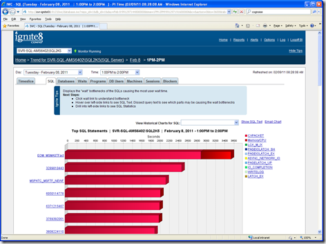
I found a query in our month end process that had a lot of CXPACKETS. This was discovered through Ignite8 from Confio. This tool brings to the top of the heap, the most costly queries based on waits. I can also just look at a day, like end of moth, or even a database among other slice and dice capabilities.
image

I took the query and placed it in SSMS, and did a Display Estimated Query Plan and got an index suggestion that would improve performance 99%. It was the Sub-Query columns, PatNo + LocationCode with Include Column ClaimDate. The new index took about 15 minutes to create on a 48 million row table, but the Cost went from 3300+ to <5. WOW!!! From a 3-4 hour data retrieval to ~1 hour and no more parallelism.

image

Thanks again Confio!!!


Bad SQL

Over the last 6 months in the BI group, I have discovered some SQL that turned bad after more and more rows accumulate in the tables that are queried. The problem with the query is that the function has to be performed on ever row.

Taking these trims out, which were not needed because it was populating a staging table, then comparing to the Fact table, reduced the TempDB usage tremendously. If you look at the SET STATISTICS IO ON values below, you can see the before and after effects.

WHERE LTrim(TRim(column) = LTrim(RTrim(column)

WORKTABLE used

Table 'Worktable'. Scan count 1929907, logical reads 33462081, physical reads 0, read-ahead reads 0, lob logical reads 0, lob physical reads 0, lob read-ahead reads 0.

Table 'Worktable'. Scan count 0, logical reads 0, physical reads 0, read-ahead reads 0, lob logical reads 0, lob physical reads 0, lob read-ahead reads 0.

Table 'AUDIT_STAGING'. Scan count 10, logical reads 193381, physical reads 161, read-ahead reads 26709, lob logical reads 0, lob physical reads 0, lob read-ahead reads 0.

Table 'AUDIT'. Scan count 6, logical reads 85351, physical reads 20, read-ahead reads 82695, lob logical reads 0, lob physical reads 0, lob read-ahead reads 0.

WHERE column = column

Removed RTrim(LTrim())

(4622 row(s) affected)

Table 'AUDIT_STAGING'. Scan count 2, logical reads 188552, physical reads 0, read-ahead reads 0, lob logical reads 0, lob physical reads 0, lob read-ahead reads 0.

Table 'AUDIT'. Scan count 2, logical reads 145602, physical reads 0, read-ahead reads 0, lob logical reads 0, lob physical reads 0, lob read-ahead reads 0.

The ‘Worktable’ was being created in TempDB, thus slowing down the query. Amazing what some investigation can do

Answer To SQLSaturday #57 Question

Hash and non-hash Aggregate Streams – Someone in the session Execution Plan Basics asked me what was the difference between these two, and I did not have an answer. Rather than trying to make something up, I told the person I did not know, explained how many different new Execution Plan objects I see all the time, and said I would find out. The SQL Community is amazing!!!

Well, Craig Freedman’s blog answers this question.

Here is a quote from him:

“Stream aggregate is great for scalar aggregates and for aggregations where we have an index to provide a sort order on the group by column(s) or where we need to sort anyhow (e.g., due to an order by clause).

The other aggregation operator, hash aggregate, is similar to hash join.  It does not require (or preserve) sort order, requires memory, and is blocking (i.e., it does not produce any results until it has consumed its entire input).  Hash aggregate excels at efficiently aggregating very large data sets.”

God Bless,

Thomas

Thursday, December 23, 2010

CXPACKET – that mysterious wait type

At my current employer, we have experience various levels of CXPACKET waits causing or thinking that is causes problems.

The first assumption we made that the CXPACKET wait was a problem came from SQL Server error message that suggested using OPTION (MAXDOP 1). Googling the details of the error, which included the words resource semaphore, was bringing up nothing. Calls to Microsoft Premier Support was not helping either. So, we changed queries that had long CXPACKET waits (some queries would never finish) or the Resource Semaphore deadlocking to use OPTION (MAXDOP 1) and we just waited for the query to run long (at least it finished). This happened to about 5 long running queries in our OLTP system when we converted to SQL Server 2005 and larger production machines.

A good read about this situation can be located here from Bart Duncan. Thanks Bart!!!

So, we thought every time we see CXPACKET waits, we had this same problem. The SQL Server community would make comments like CXPACKET is not the problem or look at your Query Plan. Tune the query, etc. etc. But I could not see the forest through the trees.

Now, after a couple of years of reading and using various tools for performance tuning, I have now realized why some in the SQL community keep saying that CXPACKET is not the problem. The problem I was having with this statement was they were either not communicating what the problem was or my limited understanding of performance tuning hindered me from comprehending the solution. And I really believed I knew what performance tuning was all about. Man, I was wrong. And finally still today I know there is more to learn.

Our OLTP system has 5 to 1 Reads to Writes. An analysis by EMC for a new VMAX gave us these statistics. This means that long processing queries were victim to this perceived notion that CXPACKET wait was our problem. This also included our OLAP system which is Cognos and I am now a member of this department. We just assumed it was a wait problem.

Adam Machanic has a great utility called sp_WhoIsActive. By default, it does not show CXPACKET waits. He also has a recorded session on Parallel Processing which I was blessed to host for Adam and the PASS Performance Virtual Chapter. He also has a series with SQL University, which I suggest reading. Also, Paul White ( Blog | Twitter ) has been trying to clue me in on CXPACKET via Twitter for sometime now. If sp_WhoIsActive is hard to understand, first start with sp_who3, another great monitoring tool. Thanks Mr. Denny

I have 2 executions of sp_whoIsAtive in my shortcuts in SSMS:

Ctrl+7 - exec dbo.[sp_WhoIsActive] '', 'session', 'Replication%', 'program'

image

Ctrl+8 - exec dbo.[sp_WhoIsActive] @filter = '', @filter_type =  'session', @not_filter = 'Replication%', @not_filter_type = 'program', @get_task_info = 2

image

The filter is for not seeing transaction replication in the view. The Ctrl+8 has the @get_task_info = 2 which shows a combination of CXPACKET and other waits associated with the SPID execution. This is really cool stuff for a DBA geek.

After reading the above links and riffling through some execution plans, I came to an ah hah moment when I saw a Display Estimated Query Plan and the Actual Query Plan not be the same. The difference included a Nested Loop in the estimate that did a Lookup and then a Hash Loop with 2 Index Scans in the actual plan.

What I came to realize was that if I tune the query and tables(indexes), parallelism sometimes goes away. Did you get that? …it goes away. Why?  Because now the actual plan does not need to run in parallel for the best plan.

Another one came when I realized the table (Fact table in a Data Warehouse with 30+ million rows) did not have a clustered index, but many non-clustered indexes. The suggested index from the Missing Index feature of SSMS showed a new Non-clustered index, when I applied it, it did not help 90+% like the missing index feature said. So, I went to the table, found the no clustered index on table, combined the surrogate keys into a clustered index and the Query Plan cost went from 1000+ to less than 50.

WOW!!! Now I get it. Thanks Adam, Paul and others for being patient with me

One more thing, I do not remember where I saw this, but in the sys.dm_os_waiting_tasks, when  exec_content_id = 0 and the wait is CXPACKET, that means the process is waiting for parallel processing to finish, and is a valid wait.

I think I will dig up some of these old query tuning experiences and try to show others through this blog what I have found. Maybe even a step by step process I go through nowadays to find problems with performance.

Now, back to the ETL on Data Marts.

God Bless,

Thomas